
 01.最小二乘法拟合 李航统计学习方法
原文链接:https://blog.csdn.net/qq_39355828/article/details/117484021 (opens new window)
# 01.最小二乘法拟合 李航统计学习方法
最小二乘法是最简单的曲线拟合方法,包含了机器学习中的主要思想。最小二乘法的公式为:
H
(
x
)
=
w
0
+
w
1
x
+
w
2
x
2
+
.
.
.
w
n
x
n
H(x)=w_0+w_1x+w_2x^2+...w_nx^n
H(x)=w0+w1x+w2x2+...wnxn
求得一组参数:
w
(
w
0
,
w
1
,
w
2
,
.
.
.
,
w
n
)
w(w_0,w_1,w_2,...,w_n)
w(w0,w1,w2,...,wn)
使得下面式子的值最小
∑
i
=
1
n
(
h
(
x
i
)
−
y
i
)
2
\sum_{i=1}^n(h(x_i)-y_i)^2
i=1∑n(h(xi)−yi)2
举例:我们用目标函数𝑦=𝑠𝑖𝑛2𝜋𝑥, 加上一个正态分布的噪音干扰,用多项式去拟合。
先使得多项式的阶数为0:取值为 [-0.01417862]
![[外链图片转存失败,源站可能有防盗链机制,建议将图片保存下来直接上传(img-hwBUJoZn-1622639895872)(C:\Users\123\AppData\Roaming\Typora\typora-user-images\1622637873568.png)]](/csdn-assets/117484021/image-01.png)
阶数为3:取值为:[ 22.66055798 -33.9628942 11.53222007 -0.12498088]
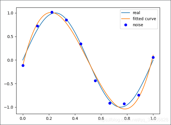
阶数为9:取值[-4.22467034e+03 2.14809765e+04 -4.56314211e+04 5.27151765e+04 -3.61213800e+04 1.50149341e+04 -3.68301369e+03 4.66946773e+02 -1.75055531e+01 -4.28685003e-02]
![[外链图片转存失败,源站可能有防盗链机制,建议将图片保存下来直接上传(img-VhTzX36W-1622639895876)(C:\Users\123\AppData\Roaming\Typora\typora-user-images\1622638061122.png)]](/csdn-assets/117484021/image-03.png)
可以看出 多项式的阶数越高,则经过的点越多,但是阶数太大,会产生的后果就是过拟合。
#使用最小二乘法拟合曲线
import matplotlib
import numpy as np
import scipy as sp
from scipy.optimize import leastsq
import matplotlib.pyplot as plt
matplotlib.use('TkAgg')
def real_func(x):#输入x后产生的真值
    return np.sin(2*np.pi*x)

def fit_func(p,x):
    #numpy.poly1d([1,2,3]) 生成  1𝑥2+2𝑥1+3𝑥0 *
    f = np.poly1d(p)
    return f(x)
def residuals_func(p,x,y):
    ret=fit_func(p,x)-y
    return ret
x=np.linspace(0,1,10)#产生0-1之间的10个点

x_points=np.linspace(0,1,1000)
#加上正态分布噪声的目标的值
y_=real_func(x)
y=[np.random.normal(0,0.1)+y1  for y1 in y_]

def fitting(M):
    #随机初始化多项式参数
    p_init = np.random.rand(M + 1)#当阶数为M时,则需要初始化M+1个参数值
    print('p_init:',p_init)
    p_lsp=leastsq(residuals_func,p_init,args=(x,y))#最小二乘法拟合,得到拟合的参数值为p_lsp

    print('Fitting Parameters:',p_lsp[0])
    #真实的值
    plt.plot(x_points,real_func(x_points),label='real')
    #拟合的值
    plt.plot(x_points,fit_func(p_lsp[0],x_points),label='fitted curve')

    plt.plot(x,y,'bo',label='noise')

    plt.legend()
    plt.show()
    return p_lsp
p_lsq_0 = fitting(9)
p_lsq_0 = fitting(3)
p_lsq_0 = fitting(5)
p_lsq_0 = fitting(7)
1
2
3
4
5
6
7
8
9
10
11
12
13
14
15
16
17
18
19
20
21
22
23
24
25
26
27
28
29
30
31
32
33
34
35
36
37
38
39
40
41
42
43
44
45
2
3
4
5
6
7
8
9
10
11
12
13
14
15
16
17
18
19
20
21
22
23
24
25
26
27
28
29
30
31
32
33
34
35
36
37
38
39
40
41
42
43
44
45
# 02.防止过拟合问题
为了防止过拟合,引入过拟合的惩罚项,如下式,当选取的模型越复杂,即W的二范数越大,对拟合时的惩罚越大
Q
(
x
)
=
∑
i
=
1
n
(
h
(
x
i
)
−
y
i
)
2
+
λ
∣
∣
w
∣
∣
2
Q(x)=\sum_{i=1}^n(h(x_i)-y_i)^2+\lambda||w||^2
Q(x)=i=1∑n(h(xi)−yi)2+λ∣∣w∣∣2
为9次拟合加上罚项
def residuals_func_regularization(p,x,y):#为最小二乘法加入罚项
    ret = fit_func(p, x) - y
    #print(ret)
    ret=np.append(ret,np.sqrt(0.001*np.square(p)))#np.square(p)可以快速获取矩阵元素的平方
    print(ret)
    return ret
p_init = np.random.rand(10)#取9次多项式作为拟合曲线,9次多项式10个参数
p_residuals=leastsq(residuals_func_regularization,p_init,args=(x,y))#最小二乘法拟合,得到拟合的参数值为p_lsp
plt.plot(x_points,real_func(x_points),label='real')
plt.plot(x_points,fit_func(p_residuals[0],x_points),label='fitting')
plt.plot(x,y,'bo',label='noise')
plt.legend()
plt.show()
1
2
3
4
5
6
7
8
9
10
11
12
13
2
3
4
5
6
7
8
9
10
11
12
13
![[外链图片转存失败,源站可能有防盗链机制,建议将图片保存下来直接上传(img-YK7eiXeC-1622639895879)(C:\Users\123\AppData\Roaming\Typora\typora-user-images\1622639584788.png)]](/csdn-assets/117484021/image-04.png)
1代码参考 https://github.com/fengdu78/lihang-code
编辑 (opens new window)
上次更新: 2026/08/11, 13:36:18